Goal:

To test whether:

in field trials, there were significantly more male P. corruscus captured in sticky traps with solvent + pheromone versus traps with solvent alone.
in laboratory bioassays, male P. corruscus spent more time with solvent + pheromone lures than lures with solvent alone.
to generate figures for the main manuscript.

#clear the workspace
rm(list = ls())

#load necessary packages
library(ggplot2)
library(dplyr)
library(kableExtra)
library(patchwork)
library(cowplot)
library(knitr)
library(ggpubr)
library(rstatix)
library(tidyr)
library(ggpubr)
library(reshape2)
library(ggpattern)

Field Trials

Pennsylvania Field Trials Data Analysis

Step 1: Load data

#load the PA data
Ecorr_Trial_df <- read.csv("Field.Data_5.14.2022.csv", header = TRUE)

#make a nice table
Ecorr_Trial_df_summary <- Ecorr_Trial_df %>%
  group_by(Treatment) %>%
  summarise(mean_males = mean(N_individuals),
            sd_males = sd(N_individuals))

#view the table           
kbl(Ecorr_Trial_df_summary, digits = c(2), col.names = c("Treatment", "Mean males captured", "SD")) %>%
  kable_classic(full_width = F, html_font = "Cambria", position = "center")

Treatment	Mean males captured	SD
Solvent	0.0	0.00
Solvent + Pheromone	14.8	5.36

Step 2: Mann Whitney U (Wilcoxon) Test

Because data not normally distributed (solvent-only are all 0), will proceed with non-parametric tests.

#wilcox test, P = 
res <- wilcox.test(N_individuals ~ Treatment, data = Ecorr_Trial_df,
            alternative = c("less"))
res

## 
##  Wilcoxon rank sum test with continuity correction
## 
## data:  N_individuals by Treatment
## W = 0, p-value = 0.003645
## alternative hypothesis: true location shift is less than 0

P = 0.003645 - yes, the control (solvent-only) treatment catches significantly fewer individuals.

Step 3: Boxplot

Graph shows N males captured in solvent-only and solvent + pheromone traps, with standard deviation. During this trial, only male specimens were caught in traps.

#make sure Treatment is a factor
Ecorr_Trial_df <- tibble(Ecorr_Trial_df)
Ecorr_Trial_df$Treatment <- factor (Ecorr_Trial_df$Treatment, levels = c("Solvent", "Solvent + Pheromone"))

#make the stat test table
#stat.test <- Ecorr_Trial_df %>%
#  wilcox_test(N_individuals ~ Treatment, alternative = c("less")) %>%
#  add_significance()
#stat.test <- stat.test %>% add_xy_position(x = "Treatment")

Ecorr_Trial_df_mod <- Ecorr_Trial_df
Ecorr_Trial_df_mod$Treatment <- gsub("Solvent", "S", Ecorr_Trial_df_mod$Treatment)
Ecorr_Trial_df_mod$Treatment <- gsub("Pheromone", "P", Ecorr_Trial_df_mod$Treatment)

#make barplot
#q <- ggbarplot(Ecorr_Trial_df_mod, 
#               x = "Treatment", 
#               y = "N_individuals", 
#               fill = "Treatment", 
#               palette = c("#ff7f00", "#377eb8"), 
#               add = "mean_sd", 
#               xlab = FALSE, 
#               ylab = "N males", 
#               font.y = c(14, "plain", "black"),
#               legend = "none", 
#               ylim = c(0, 30))
#add stats
#q_w_sig <- q + stat_pvalue_manual(stat.test, 
#                       label = "p.signif",
#                       vjust = -1, 
#                       bracket.nudge.y = 1, 
#                       bracket.size = .7)
#q_w_sig

q_w_sig <- ggplot(Ecorr_Trial_df_mod, aes(x = Treatment, y = N_individuals, fill = Treatment)) +
  geom_boxplot(outlier.shape = NA, alpha = 0.7) +
  theme_classic() +
  xlab("Treatment") +
  ylab("N males") +
  theme(legend.position = "none", 
        axis.title.x = element_blank()) +
  scale_fill_manual(values = c("#ff7f00", "#377eb8")) +
  ylim(c(-1,30))+
  geom_jitter(alpha = 0.9) +
  geom_signif(comparisons=list(c("S", "S + P")), annotations="**",
              y_position = 25, tip_length = .01, vjust=0.4)
q_w_sig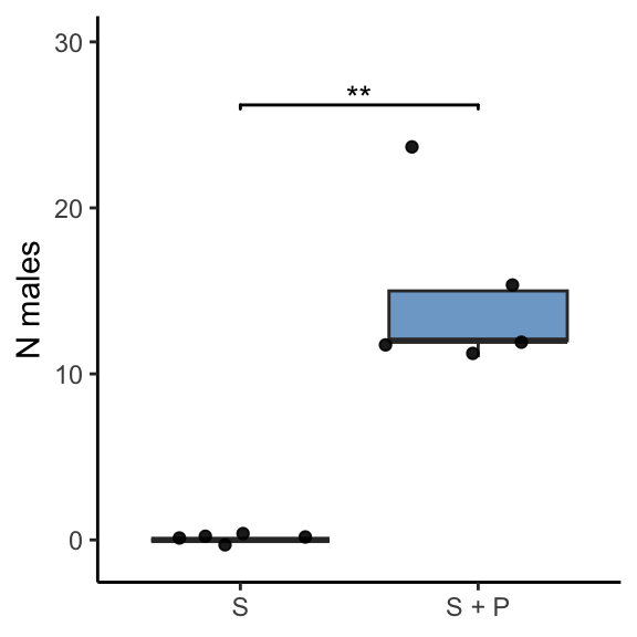

#ggsave("PA_field_trials_2022.pdf", q_w_sig, device = "pdf", width = 58, height = 65, units = c("mm"), dpi = 1200)
#ggsave("PA_field_trials_2022.png", q_w_sig, device = "png", width = 58, height = 65, units = c("mm"), dpi = 1200)

Vermont Field Trials Data Analysis

Step 1: Input VT Data

#load the PA data
VT_Ecorr_Trial_df <- read.csv("VT_Field.Data_5.20.2022.csv", header = TRUE)

#make a nice table
VT_Ecorr_Trial_df_summary <- VT_Ecorr_Trial_df %>%
  group_by(Treatment) %>%
  summarise(mean_males = mean(N_individuals),
            sd_males = sd(N_individuals))

#view the table           
kbl(VT_Ecorr_Trial_df_summary, digits = c(2), col.names = c("Treatment", "Mean males captured", "SD")) %>%
  kable_classic(full_width = F, html_font = "Cambria", position = "center")

Treatment	Mean males captured	SD
Solvent	0	0.00
Solvent + Pheromone	9	4.64

Step 2: Mann Whitney U (Wilcoxon) Test

Because data not normally distributed (solvent-only are all 0), will proceed with non-parametric tests.

#wilcox test, P = 
res <- wilcox.test(N_individuals ~ Treatment, data = VT_Ecorr_Trial_df,
            alternative = c("less"))
res

## 
##  Wilcoxon rank sum test with continuity correction
## 
## data:  N_individuals by Treatment
## W = 0, p-value = 0.003645
## alternative hypothesis: true location shift is less than 0

P = 0.003645 - yes, the control (solvent-only) treatment catches significantly fewer individuals.

Step 3: Boxplot

Graph shows N males for control and treatment groups, with standard deviation. During this trial, only male specimens were caught in traps.

#make sure Treatment is a factor
VT_Ecorr_Trial_df <- tibble(VT_Ecorr_Trial_df)
VT_Ecorr_Trial_df$Treatment <- factor (VT_Ecorr_Trial_df$Treatment, levels = c("Solvent", "Solvent + Pheromone"))

#make the stat test table
#stat.test <- VT_Ecorr_Trial_df %>%
#  wilcox_test(N_individuals ~ Treatment, alternative = c("less")) %>%
#  add_significance()
#stat.test <- stat.test %>% add_xy_position(x = "Treatment")

#change treatment labels to be more compact
VT_Ecorr_Trial_df_mod <- VT_Ecorr_Trial_df
VT_Ecorr_Trial_df_mod$Treatment <- gsub("Solvent", "S", VT_Ecorr_Trial_df_mod$Treatment)
VT_Ecorr_Trial_df_mod$Treatment <- gsub("Pheromone", "P", VT_Ecorr_Trial_df_mod$Treatment)

#make barplot
#r <- ggbarplot(VT_Ecorr_Trial_df_mod, 
#               x = "Treatment", 
#               y = "N_individuals", 
#               fill = "Treatment", 
#               palette = c("black", "white"), 
#               add = "mean_sd", 
#               xlab = FALSE, 
#               ylab = "N males", 
#               font.y = c(14, "plain", "black"),
#               legend = "none", 
#               ylim = c(0, 30))
#add stats
#r_w_sig <- r + stat_pvalue_manual(stat.test, 
#                       label = "p.signif",
#                       vjust = -1, 
#                       bracket.nudge.y = 1, 
#                       bracket.size = .7)
#r_w_sig

r_w_sig <- ggplot(VT_Ecorr_Trial_df_mod, aes(x = Treatment, 
                           y = N_individuals)) +
  geom_boxplot_pattern(aes(pattern_fill = Treatment),
                       fill = c("#ff7f00", "#377eb8"),
                       color = "black",
                       pattern = 'stripe',
                       pattern_fill = "black") +
  theme_classic() +
  xlab("Treatment") +
  ylab("N males") +
  theme(legend.position = "none", 
        axis.title.x = element_blank()) +
  ylim(c(-2,30)) +
  geom_jitter(alpha = 0.9) +
  geom_signif(comparisons=list(c("S", "S + P")),
              annotations="**",
              y_position = 25, 
              tip_length = .01, 
              vjust=0.4)

r_w_sig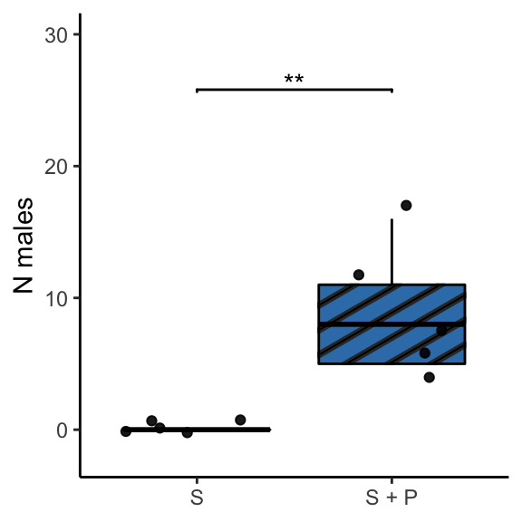

#ggsave("VT_field_trials_2022.pdf", r_w_sig, device = "pdf", width = 58, height = 65, units = c("mm"), dpi = 1200)
#ggsave("VT_field_trials_2022.png", r_w_sig, device = "png", width = 58, height = 65, units = c("mm"), dpi = 1200)

Lab Trials

Step 1: Read in the data

All Data (N unique males = 8)

#read in data
Behavioral_Analysis <- read.csv("Behavioral_Analysis_Sheet_Rep1.csv", header = TRUE)

#get data into usable form
Behavioral_Analysis_raw <- tibble(Filename = Behavioral_Analysis$File_Name, Male = Behavioral_Analysis$Male, Duration = Behavioral_Analysis$Total_time_of_behavior_s, Behavior = Behavioral_Analysis$Behavior)

#Sum behaviors by each male
Behavioral_Analysis_summary <- Behavioral_Analysis_raw %>%
  group_by(Male, Behavior) %>%
  summarize(Cumulative_time_s = sum(Duration))

#Make longer to figure out where there are instances of no contact in control or experimental -> replace with 0s
Behavioral_Analysis_summary_wide <- Behavioral_Analysis_summary %>%
  pivot_wider(names_from = Behavior, values_from = Cumulative_time_s)

#Change NAs to zero (if a behavior didn't happen, it wasn't logged)
Behavioral_Analysis_summary_wide <- Behavioral_Analysis_summary_wide %>%
  mutate_at(vars(c("TOUCHING_E", "TOUCHING_C", "MOUNTING_E", "MOUNTING_C", "COPULATING_E")), ~replace_na(.,0))

#There were no copulations with control -> add a column for that
Behavioral_Analysis_summary_wide$COPULATING_C <- 0

#add in columns for total contact time with experimental and control
Behavioral_Analysis_summary_wide <-
  Behavioral_Analysis_summary_wide %>%
  mutate(Total_contact_time_E = sum(TOUCHING_E, MOUNTING_E, COPULATING_E),
         Total_contact_time_C = sum(TOUCHING_C, MOUNTING_C, COPULATING_C))

#convert to long form
Behavioral_Analysis_summary_long <-
  Behavioral_Analysis_summary_wide %>%
  pivot_longer(cols = c("TOUCHING_E", "TOUCHING_C", "MOUNTING_E", "MOUNTING_C", "COPULATING_E", "COPULATING_C", "Total_contact_time_E", "Total_contact_time_C"), 
               names_to = "Behavior_by_trap_type", 
               values_to = "Time")
  
#Separate Behavior column into trap type and behavior
Behavioral_Analysis_summary_long <- Behavioral_Analysis_summary_long %>%
  mutate(Behavior = case_when(
    startsWith(Behavior_by_trap_type, "TOUCHING") ~ "Touching",
    startsWith(Behavior_by_trap_type, "MOUNTING") ~ "Mounting",
    startsWith(Behavior_by_trap_type, "COPULATING") ~ "Copulating",
    startsWith(Behavior_by_trap_type, "Total") ~ "Contact"
    ),
    Trap_type = case_when(
      endsWith(Behavior_by_trap_type, "E") ~ "Solvent + Pheromone",
      endsWith(Behavior_by_trap_type, "C") ~ "Solvent"
    ))

#sum time by male and treatment (trap_type)
first_rep_data_by_male <- Behavioral_Analysis_summary_long %>%
  group_by(Male, Trap_type, Behavior) %>%
  summarize(Time_spent = sum(Time))

#calculate means and std_dev
first_reps_mean_std <- first_rep_data_by_male %>%
  group_by(Trap_type, Behavior) %>%
  summarise(mean_time = mean(Time_spent)/60, std_dev = sd(Time_spent)/60)

#make variable that combines the two
first_reps_mean_std <- first_reps_mean_std %>%
  mutate(Mean_SD = paste0(round(mean_time,2), " (", round(std_dev, 2), ")"))

#select just desired columns
first_reps_mean_std_wide <- first_reps_mean_std[,c(1,2,5)] %>%
  spread(Behavior, Mean_SD)

#reorder the columns
first_reps_mean_std_wide_ordered <- first_reps_mean_std_wide[,c(1,5,4,3,2)]

#control data by itself
control_data_by_male <- first_rep_data_by_male %>%
  spread(Behavior, Time_spent) %>%
  filter(Trap_type == "Solvent")

control_data_by_male_ordered <- control_data_by_male[,c(1,2,6,5,4,3)]

#experimental data by itself
experimental_data_by_male <- first_rep_data_by_male %>%
  spread(Behavior, Time_spent) %>%
  filter(Trap_type == "Solvent + Pheromone")

experimental_data_by_male_ordered <- experimental_data_by_male[,c(1,2,6,5,4,3)]

#display means + sds as kable
big_table <- kbl(first_reps_mean_std_wide_ordered) %>%
  kable_classic(full_width = F, html_font = "Cambria", position = "center")
big_table <- add_header_above(big_table, c(" ", "Mean time (sd)*" = 4))
big_table <- add_footnote(big_table, c(paste0("in minutes; N males = ", nrow(control_data_by_male))), notation = "symbol")
big_table

	Mean time (sd)*
Trap_type	Touching	Mounting	Copulating	Contact
Solvent	0.08 (0.18)	0.04 (0.08)	0 (0)	0.12 (0.25)
Solvent + Pheromone	1.74 (3.72)	1.12 (1.78)	0.05 (0.09)	2.91 (3.63)
^* in minutes; N males = 8

Note: All means are smaller for Control traps when compared to experimental (pheromone) traps. However, the standard deviations are large.

Step 2: Statistical Tests

Total time in contact

1. Are the data normally distributed?

#1 - is data normally distributed?
contact_data <- first_rep_data_by_male %>%
  filter(Behavior == "Contact")

contact_data$Male <- factor(contact_data$Male, levels =  unique(contact_data$Male))

ggplot(contact_data, aes(x = Time_spent/60)) +
  geom_histogram() +
  theme_classic() +
  labs(x = "Time spent (min)", y = "N fireflies")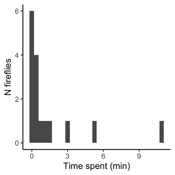

#nope
shapiro.test(contact_data$Time_spent/60)

## 
##  Shapiro-Wilk normality test
## 
## data:  contact_data$Time_spent/60
## W = 0.59089, p-value = 1.33e-05

No. Shapiro-Wilk test < 0.05. Try log-transforming.

2. After square-root transformation, are the data normally distributed?

#try log-transform
contact_data <- contact_data %>%
  mutate(sqrtCDmin = sqrt(Time_spent/60))

#looks better -> a lot of zeros
ggplot(contact_data, aes(x = sqrtCDmin)) +
  geom_histogram() +
  theme_classic() +
  labs(x = "Square-root Time spent (min)", y = "N fireflies")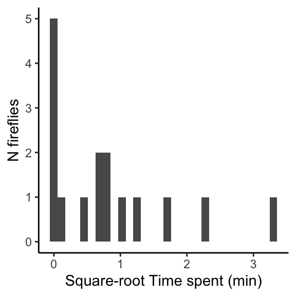

#nope
shapiro.test(contact_data$sqrtCDmin)

## 
##  Shapiro-Wilk normality test
## 
## data:  contact_data$sqrtCDmin
## W = 0.83253, p-value = 0.007616

No. Shapiro-Wilk test < 0.05, even after square-root transform -> lots of zeros, especially in control. Proceed with non-parametrics.

3. Do males spend more time in contact with lures with pheromone? (nonparametric)

Paired wilcox test

#do non-parametric test
#wilcox.test in R contains a "paired" option. 
#p = 0.003906
wilcox.test(Time_spent ~ Trap_type, data=contact_data, alternative = c("less"), paired = TRUE)

## 
##  Wilcoxon signed rank exact test
## 
## data:  Time_spent by Trap_type
## V = 0, p-value = 0.003906
## alternative hypothesis: true location shift is less than 0

P = 0.003906 - yes, significantly less time spent in contact with solvent-only lures

4. Visualizing the data

Just contact

#plotting contact
t_w_sig <- ggplot(contact_data, aes(x = Trap_type, y = Time_spent/60, fill = Trap_type)) +
  geom_boxplot(outlier.shape = NA) +
  geom_jitter(aes(x = Trap_type, y = Time_spent/60)) +
  ylab("Time (min)") +
  ylim(c(-0.5, 12)) +
  theme_classic() +
  theme(axis.title.x = element_blank(), legend.position = "none") +
  scale_x_discrete(labels = c("S", "S + P")) +
  scale_fill_manual(values = c("#377eb8", "#ff7f00")) +
  geom_signif(comparisons=list(c("Control", "Experimental")), annotations="**",
              y_position = 11, tip_length = .01, vjust=0.4)

t_w_sig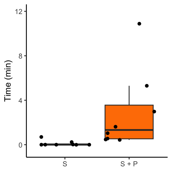

#ggsave("contact.pdf", t_w_sig, device = "pdf", width = 58, height = 65, units = c("mm"), dpi = 1200)
#ggsave("contact.png", t_w_sig, device = "png", width = 58, height = 65, units = c("mm"), dpi = 1200)

Another way to view the data (looking at pairs)

#plot pairs
ggplot(contact_data, aes(x = Trap_type, y = Time_spent/60, color = Male, group = Male)) +
  geom_point() +
  geom_line() +
  scale_color_manual(values = c("#a6cee3", "#1f78b4", "#b2df8a", "#33a02c", "#fb9a99", "#e31a1c", "#fdbf6f", "#ff7f00")) +
  theme_classic() +
  ylab("Time (min)") +
  theme(axis.title.x=element_blank()) +
  scale_x_discrete(labels = c("S", "S + P"))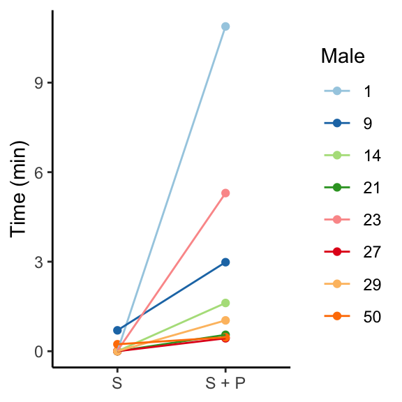

By different behaviors

Contact and other data, broken down by behavior type: the big plot

# big plot
first_rep_data_by_male_just_types<- first_rep_data_by_male %>%
  filter(Behavior == "Touching" | Behavior == "Mounting" | Behavior == "Copulating")
  
ggplot(first_rep_data_by_male_just_types, aes(x = Trap_type, y= Time_spent/60, fill = Trap_type, color = Trap_type)) +
  geom_boxplot(outlier.shape = NA, alpha = 0.25) +
  geom_jitter(aes(x = Trap_type, y = Time_spent/60)) +
  facet_grid(~Behavior) +
  theme_classic() +
  scale_x_discrete(labels = c("S", "S + P")) +
  theme(axis.title.x=element_blank(), legend.position = "none") +
  ylab("Time (min)") +
  scale_color_manual(values = c("#E8751E", "#007AAE")) +
  scale_fill_manual(values = c("#E8751E", "#007AAE"))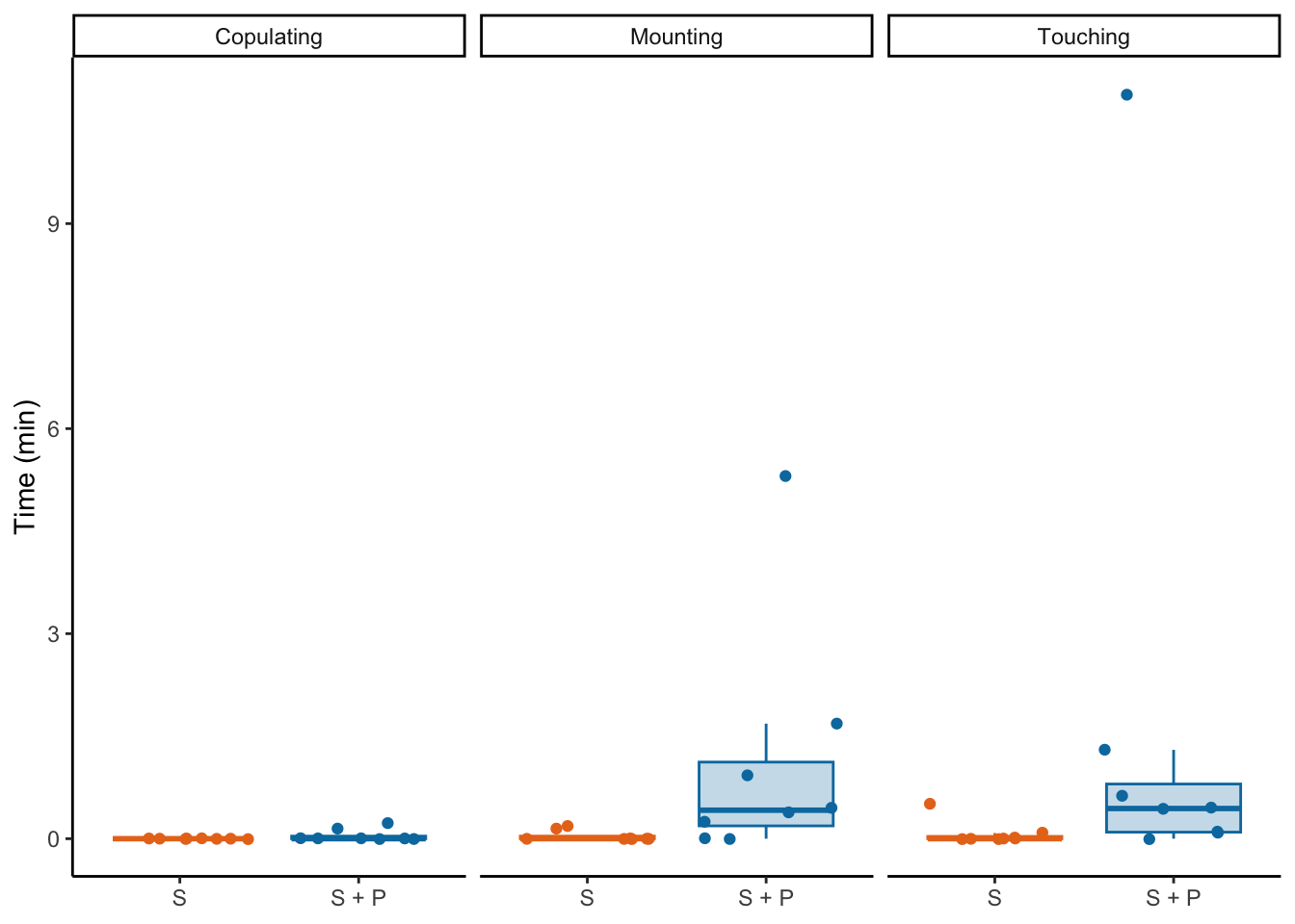

1. Does the difference in time spent between control and pheromone traps differ among behavioral types?

Friedman test of differences by behavioral type

first_rep_data_by_male$Behavior <- factor(first_rep_data_by_male$Behavior, levels =  c("Touching", "Mounting", "Copulating", "Contact"))

first_rep_data_by_male$Male <- factor(first_rep_data_by_male$Male, levels = unique(first_rep_data_by_male$Male))

#generate data table with pairs
contact_data2 <- first_rep_data_by_male %>%
  filter(Behavior == "Contact") %>%
  spread(key = Trap_type, value = Time_spent)

touch_data2 <- first_rep_data_by_male %>%
  filter(Behavior == "Touching") %>%
  spread(key = Trap_type, value = Time_spent)

mount_data2 <- first_rep_data_by_male %>%
  filter(Behavior == "Mounting") %>%
  spread(key = Trap_type, value = Time_spent)

copulate_data2 <- first_rep_data_by_male %>%
  filter(Behavior == "Copulating") %>%
  spread(key = Trap_type, value = Time_spent)

diff_df2 <- tibble(Male = contact_data2$Male, Diff_touch = (touch_data2$`Solvent + Pheromone` - touch_data2$Solvent)/60, Diff_mount = (mount_data2$`Solvent + Pheromone` = mount_data2$Solvent)/60, Diff_copulate = (copulate_data2$`Solvent + Pheromone` - copulate_data2$Solvent)/60, Diff_contact = (contact_data2$`Solvent + Pheromone` - contact_data2$Solvent)/60)

#try just looking at diffs
df_freid <- diff_df2 %>%
  melt(id.vars= c("Male"), measure.vars = c("Diff_touch", "Diff_mount", "Diff_copulate", "Diff_contact")) %>%
  filter(variable == "Diff_touch" | variable == "Diff_mount" | variable == "Diff_copulate")

df_freid$Male <- factor(df_freid$Male, levels = unique(df_freid$Male))
df_freid$variable <- factor(df_freid$variable, levels = c("Diff_touch", "Diff_mount", "Diff_copulate"))

friedman.test(y=df_freid$value, group=df_freid$variable, blocks=df_freid$Male)

## 
##  Friedman rank sum test
## 
## data:  df_freid$value, df_freid$variable and df_freid$Male
## Friedman chi-squared = 4.5185, df = 2, p-value = 0.1044

#NS - p = 0.1044

No, there is not a significant difference in the amount of time spent near pheromone vs solvent across behavioral types.
Visualization

long_df <- diff_df2 %>%
  melt(id.vars= c("Male"), measure.vars = c("Diff_touch", "Diff_mount", "Diff_copulate", "Diff_contact"))

long_df <- long_df %>%
  filter(variable == "Diff_touch" | variable == "Diff_mount" | variable == "Diff_copulate")

ggplot(long_df, aes(x = variable, y = value, color = Male)) +
  geom_point(alpha = 0.8) +
  theme_classic() +
  scale_color_manual(values = c("#a6cee3", "#1f78b4", "#b2df8a", "#33a02c", "#fb9a99", "#e31a1c", "#fdbf6f", "#ff7f00")) +
  theme(legend.position = "none") +
  labs(x = "Behavior", y = "Difference in time spent (min)") +
  geom_hline(yintercept = 0, lty = 5, color = "grey") +
  scale_x_discrete(labels = c("Touching", "Mounting", "Copulating", "Contact")) +
  ylim(-1,11)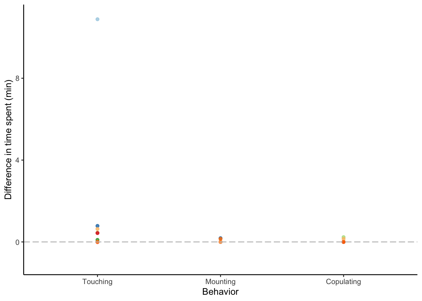

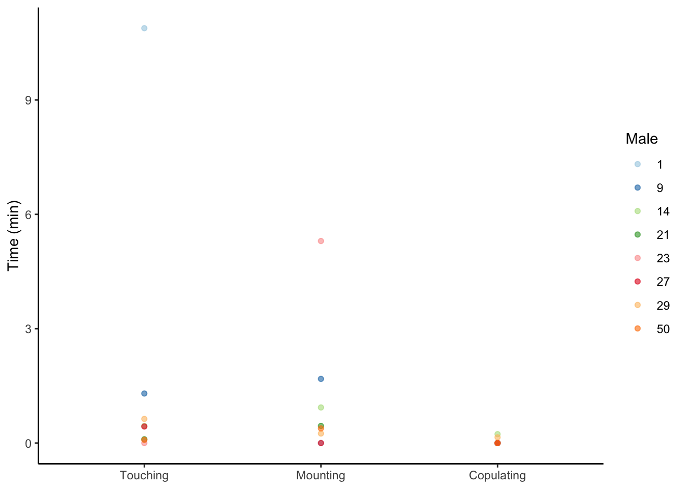
2. Does the time spent at the pheromone trap significantly differ among behavioral types?

Friedman test of time @ pheromone trap by behavioral type

#isolate just behaviors, NOT their summation (contact)
first_rep_data_by_male_subset <- first_rep_data_by_male %>%
  filter(Behavior == "Touching" | Behavior == "Mounting" | Behavior == "Copulating")

#isolate just the experimental results
first_rep_data_by_male_subset_exp <- first_rep_data_by_male_subset %>%
  filter(Trap_type == "Solvent + Pheromone")

#make sure male (block) is a factor
first_rep_data_by_male_subset_exp$Male <- factor(first_rep_data_by_male_subset_exp$Male)

#make sure behavior (explanatory variable) is a factor
first_rep_data_by_male_subset_exp$Behavior <- factor(first_rep_data_by_male_subset_exp$Behavior, levels = c("Touching", "Mounting", "Copulating"))

#friedman test
friedman.test(y=first_rep_data_by_male_subset_exp$Time_spent, group=first_rep_data_by_male_subset_exp$Behavior, blocks=first_rep_data_by_male_subset_exp$Male)

## 
##  Friedman rank sum test
## 
## data:  first_rep_data_by_male_subset_exp$Time_spent, first_rep_data_by_male_subset_exp$Behavior and first_rep_data_by_male_subset_exp$Male
## Friedman chi-squared = 8.8966, df = 2, p-value = 0.0117

#pairwise wilcox follow-up
pairwise.wilcox.test(first_rep_data_by_male_subset_exp$Time_spent, first_rep_data_by_male_subset_exp$Behavior, p.adj = "BH")

## 
##  Pairwise comparisons using Wilcoxon rank sum test with continuity correction 
## 
## data:  first_rep_data_by_male_subset_exp$Time_spent and first_rep_data_by_male_subset_exp$Behavior 
## 
##            Touching Mounting
## Mounting   1.000    -       
## Copulating 0.024    0.024   
## 
## P value adjustment method: BH

Visualization
- First, the overall plot and stats

ggplot(first_rep_data_by_male_subset_exp, aes(x = Behavior, y = Time_spent/60)) +
  geom_boxplot() +
  theme_classic() +
  ylab("Time (min)") +
  theme(axis.title.x = element_blank()) +
  geom_signif(comparisons=list(c("Mounting", "Copulating")), annotations="*",
              y_position = 11, tip_length = .01, vjust=0.4) +
  geom_signif(comparisons=list(c("Touching", "Copulating")), annotations="*",
              y_position = 12, tip_length = .01, vjust=0.4)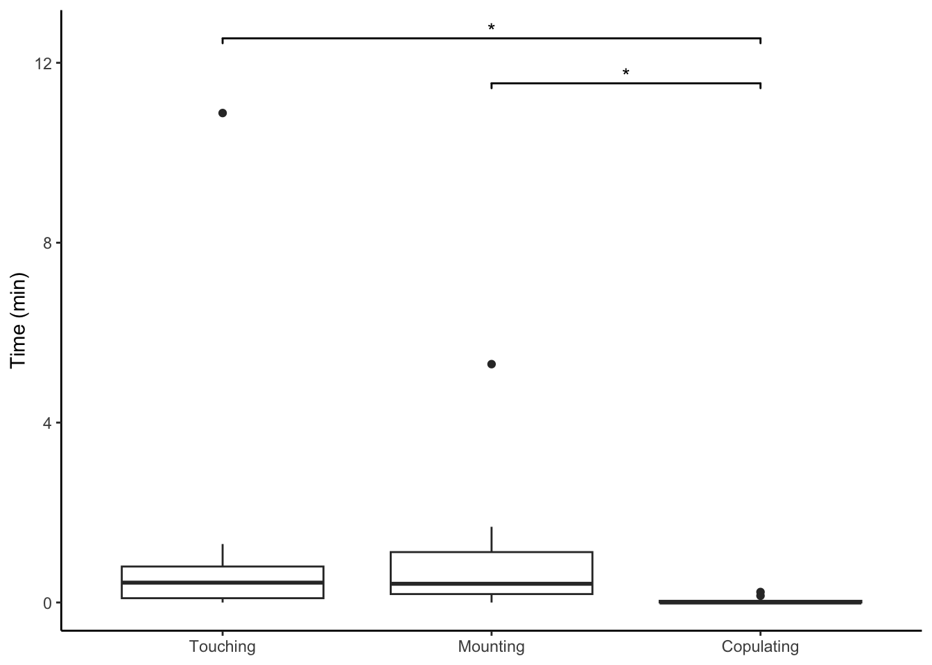

Then, by pairs

ggplot(first_rep_data_by_male_subset_exp, aes(x = Behavior, y = Time_spent/60, color = Male)) +
  geom_point(alpha= 0.6) +
  theme_classic() +
  ylab("Time (min)") +
  theme(axis.title.x = element_blank()) +
  scale_color_manual(values = c("#a6cee3", "#1f78b4", "#b2df8a", "#33a02c", "#fb9a99", "#e31a1c", "#fdbf6f", "#ff7f00"))

Field Trial Statistics

Hannah Holmes and Dr. Sarah Lower

5/15/2022

Goal:

Field Trials

Pennsylvania Field Trials Data Analysis

Step 1: Load data

Step 2: Mann Whitney U (Wilcoxon) Test

Step 3: Boxplot

Vermont Field Trials Data Analysis

Step 1: Input VT Data

Step 2: Mann Whitney U (Wilcoxon) Test

Step 3: Boxplot

Lab Trials

Step 1: Read in the data

Step 2: Statistical Tests

Total time in contact

1. Are the data normally distributed?

2. After square-root transformation, are the data normally distributed?

3. Do males spend more time in contact with lures with pheromone? (nonparametric)

4. Visualizing the data

By different behaviors

1. Does the difference in time spent between control and pheromone traps differ among behavioral types?

2. Does the time spent at the pheromone trap significantly differ among behavioral types?